Decision Trees

A decision tree predicts by routing an example through feature-threshold tests until it reaches a leaf. It is the base learner behind random forests and most classical gradient boosting systems.

How a tree is built

A decision tree is grown greedily, one split at a time, by recursively partitioning the training data. Each split asks for the single question — one feature, one threshold — that makes the two children purer than the parent:

1. Start at the root with all training samples in a single node.
2. Search candidate splits. For every feature and every candidate threshold, consider dividing the node’s samples into a left group (feature below the threshold) and a right group (at or above it).
3. Score each split by how much purer the two children are than the parent — the impurity decrease $\Delta$ defined below. “Pure” means one class dominates (classification) or the target has low variance (regression).
4. Keep the best split, the one with the largest $\Delta$, and attach its two children to the node.
5. Recurse on each child, using only the samples routed to it.
6. Stop when a rule fires — maximum depth reached, too few samples to split further, or a node already pure — and turn the node into a leaf.

Prediction is then a lookup: route a new example down the threshold tests until it reaches a leaf, and return that leaf’s majority class (classification) or mean target (regression). Each root-to-leaf path is an axis-aligned if-then rule, which is what makes trees easy to read with interpretability tools — but also unstable, because a slightly different sample can change an early split and reshape the whole subtree.

Splitting criteria

Step 3 needs a measure of node impurity. For classification, consider a node $m$ holding a subset of the training samples, and let $p_{mk}$ be the proportion of those samples that belong to class $k$. The node’s impurity can be measured by Gini impurity $G_m=1-{\sum }_k{p}_{mk}^2$ or entropy $H_m=-{\sum }_k{p}_{mk}\log p_{mk}$; both are largest when classes are evenly mixed and zero when the node contains a single class. A candidate split $s$ divides node $m$ into a left and a right child, and is scored by the impurity decrease it produces:

$$\Delta (s,m)=I_m-\frac{n_L}{n_m}{I}_L-\frac{n_R}{n_m}{I}_R,$$

where $I_m$ is the impurity of node $m$ (Gini, entropy, or — for regression trees — the within-node variance of the target), $n_m$ is the number of samples at the node, $n_L$ and $n_R$ are the counts sent to the left and right children, and $I_L$, $I_R$ are those children’s impurities. The tree keeps the split with the largest $\Delta$, and the prediction at a leaf is the majority class or mean target of the samples that reach it.

Worked example

This is a binary classification example, where a split is scored by how pure it makes the resulting groups. Consider a node holding ten training samples, five from the positive class and five from the negative class, so each class proportion is $p_{mk}=\frac{5}{10}$. Its Gini impurity $G_{\text{parent}}$ is

$$G_{\text{parent}}=1-{\left(\frac{5}{10}\right)}^2-{\left(\frac{5}{10}\right)}^2=0.5,$$

the maximum for a two-class node, because the classes are perfectly mixed. A candidate split on feature $x_2$ at threshold $t$ sends $n_L=4$ samples to the left child (all positive) and $n_R=6$ to the right child (one positive, five negative), whose impurities $G_L$ and $G_R$ are

$$G_L=1-1^2-0^2=0,G_R=1-{\left(\frac{1}{6}\right)}^2-{\left(\frac{5}{6}\right)}^2=\frac{10}{36}\approx \mathrm{0.278.}$$

Weighting each child impurity by its share of the $n_m=10$ samples ($n_L/n_m$ and $n_R/n_m$) gives the split impurity, and the impurity decrease $\Delta$ is the parent impurity minus that weighted child impurity:

$$\frac{4}{10}(0)+\frac{6}{10}(0.278)=0.167,\Delta =0.5-0.167=\mathrm{0.333.}$$

The tree keeps the split with the largest $\Delta$, then recurses on each child until a stopping rule fires. The left child is already pure, so it becomes a leaf; the right child can be split again on another feature:

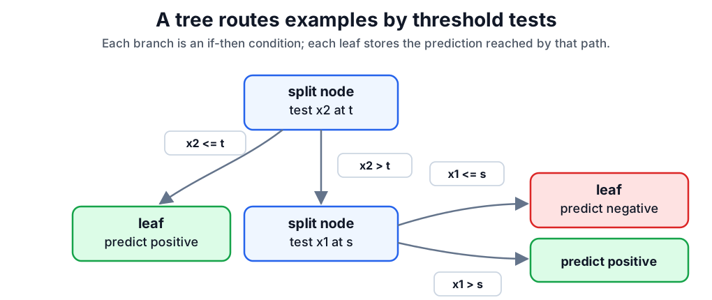
Each path from root to leaf is an if-then rule built from axis-aligned threshold tests, and a prediction is simply the majority class (or mean target) of the leaf an example reaches.

Caveats

Deep unpruned trees have low bias and high variance, which is why they are often averaged in random forests. Axis-aligned splits can approximate curved boundaries only with many rectangles. Standard impurity-based feature importance can favor continuous or high-cardinality features.

References

• scikit-learn User Guide: Decision Trees
• An Introduction to Statistical Learning

Nav

Section — Classical Machine Learning

← Feature Engineering Random Forests →