Regularization

Regularization changes the training problem so a model must buy fit with complexity. In linear models this usually means shrinking coefficients; with lasso, it can also prune features by driving some coefficients exactly to zero. In gradient boosting, regularization means small learning rates, shallow trees, subsampling, and early stopping. Neural networks use the same principle, but with additional mechanisms such as dropout, data augmentation, and weight decay; see deep-learning regularization.

Defining math

A regularized estimator adds a complexity penalty to the average training loss:

$$\hat{\theta }=\arg \underset{\theta }{\min }\frac{1}{n}\sum _{i=1}^{n}L(y_i,f_{\theta }(x_i))+\lambda \Omega (\theta ),$$

where $\theta$ are the model parameters, $f_{\theta }$ is the model, $L$ is the per-example loss over the $n$ training examples, $\Omega (\theta )$ measures model complexity, and $\lambda \ge 0$ is the penalty strength that trades fit against simplicity. Ridge uses the squared ${\ell }_2$ norm $\Omega (\beta )=\Vert \beta {\Vert }_2^2$, giving the closed-form linear estimator ${\hat{\beta }}_{ridge}=(X^{\top }X+\lambda I{)}^{-1}{X}^{\top }y$ (with $I$ the identity matrix). The lasso uses the ${\ell }_1$ norm $\Omega (\beta )=\Vert \beta {\Vert }_1={\sum }_j|{\beta }_j|$, which can set coefficients exactly to zero. A zero coefficient removes that feature from the fitted linear prediction, so lasso is both a regularizer and a simple embedded feature-selection method. For logistic regression, the same penalties apply to cross-entropy rather than squared error.

The same idea can be drawn as a constrained problem:

$$\underset{\beta }{\min }\text{loss}(\beta )\text{subject to}\Omega (\beta )\le c.$$

The penalty form and constrained form are two views of the same trade-off: larger $\lambda$ corresponds to a tighter effective constraint. This constrained view explains why ridge shrinks and lasso can prune. In neural networks, the same penalty view appears most directly as weight decay, while stochastic methods such as dropout are regularizers that are not just coefficient penalties.

Intuition

Regularization encodes skepticism. A large coefficient, deep tree, or late boosting stage must improve validation loss enough to justify the added sensitivity. This is why regularization belongs with the bias-variance trade-off: it often increases bias slightly to reduce variance substantially.

Ridge and lasso express that skepticism differently. Ridge keeps every feature but makes large coefficients expensive, which is useful when many small signals may matter or predictors are correlated. Lasso charges a flat cost for moving each coefficient away from zero, so weak or redundant features often stay at exactly zero. In practice, those zeroed coefficients are feature pruning: the trained model ignores those columns at prediction time.

Worked example

Regularization shrinks coefficients toward zero, and in the one-feature case ridge does so with an exact closed form. With $X^{\top }X=10$ and $X^{\top }y=20$, ordinary least squares gives $\hat{\beta }=20/10=2$. Ridge divides by $X^{\top }X+\lambda$ instead:

$${\hat{\beta }}_{\text{ridge}}=\frac{X^{\top }y}{X^{\top }X+\lambda }=\frac{20}{10+\lambda }\Rightarrow \lambda =10\to 1.0,\lambda =40\to \mathrm{0.4.}$$

Larger $\lambda$ shrinks the coefficient smoothly toward zero but never exactly to zero.

For two coefficients, the constrained view gives the geometry in the diagram. The orange ellipses are loss contours: every point on the same ellipse has the same training loss, and the ellipse center is the unconstrained ordinary least squares solution ${\hat{\beta }}_{\text{OLS}}$. Without regularization, the model chooses that center. With regularization, the model must choose a point inside the blue constraint region, so the solution is the point with the lowest possible loss that still satisfies the constraint.

To find it visually, start at ${\hat{\beta }}_{\text{OLS}}$ and move outward to higher-loss contours until one first touches the blue shape. That first touching point is the regularized estimate. Ridge uses the circular ${\ell }_2$ constraint ${\beta }_1^2+{\beta }_2^2\le c$, whose smooth boundary usually touches a contour away from the axes. Both coefficients are shrunk, but both remain nonzero. Lasso uses the diamond-shaped ${\ell }_1$ constraint $|{\beta }_1|+|{\beta }_2|\le c$, whose sharp corners lie on the axes. A contour often touches one of those corners first, and a corner means one coefficient is exactly zero:

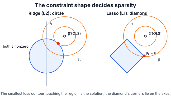
That geometric difference is why the lasso doubles as feature selection while ridge only stabilizes. If ${\beta }_j=0$, feature $x_j$ contributes nothing to $x^{\top }\beta$; after fitting, the model has effectively pruned that feature.

Comparing ridge and lasso

On real data the difference shows up as a coefficient count: the lasso zeroes some out, ridge keeps them all, and which wins on held-out error depends on the problem.

from sklearn.datasets import make_regression
from sklearn.linear_model import LinearRegression, Ridge, Lasso
from sklearn.metrics import mean_squared_error
from sklearn.model_selection import train_test_split
import numpy as np
 
X, y, _ = make_regression(n_samples=100, n_features=8, n_informative=3,
                          noise=25, coef=True, random_state=3)
Xtr, Xte, ytr, yte = train_test_split(X, y, random_state=3)
for est in [LinearRegression(), Ridge(alpha=20), Lasso(alpha=2, max_iter=10000)]:
    est.fit(Xtr, ytr)
    rmse = mean_squared_error(yte, est.predict(Xte)) ** 0.5
    print(est.__class__.__name__, "rmse", round(rmse, 2),
          "nonzero", int(np.sum(np.abs(est.coef_) > 1e-6)))

Observed output:

LinearRegression rmse 23.75 nonzero 8
Ridge rmse 24.07 nonzero 8
Lasso rmse 23.33 nonzero 7

The lasso removes one coefficient and slightly improves this held-out RMSE. That does not prove lasso is universally better; it shows how a sparsity penalty can trade a little fit flexibility for stability and produce a smaller active feature set.

Caveats

The scale of features changes the effective penalty, so standardize numeric predictors before comparing coefficients. Regularization strength is a hyperparameter and belongs inside model selection, not on the test set. Lasso feature pruning is unstable when predictors are strongly correlated: it may keep one feature from a correlated group and drop another even when both carry similar signal. Ridge is usually more stable but not sparse.

References

• scikit-learn User Guide: Ridge regression and Lasso
• Tibshirani, 1996, Regression Shrinkage and Selection via the Lasso

Nav

Section — Classical Machine Learning

← Support Vector Machines Bias-Variance Trade-Off →