Common Distributions

A probability distribution assigns mass or density to the values of a random variable. The useful part is not the name; it is the data-generating mechanism. Bernoulli and binomial laws describe independent yes/no trials, multinomial laws describe categorical counts, Poisson laws describe counts under a constant rate, normal laws describe symmetric additive noise, and gamma or exponential laws describe positive waiting-time-like quantities.

Distribution choice directly affects maximum likelihood, expectation and variance, central limit theorem approximations, and the null models used in hypothesis testing. A test statistic is only meaningful after its observation model and reference distribution have been specified.

Matching laws to mechanisms

Use the support first. Binary outcomes, nonnegative counts, positive waiting times, real-valued errors, and proportions live on different sample spaces. Then check the mechanism: independent trials, fixed margins, additive noise, and estimated variance all imply different distributions.

Distribution	What it models	Mean	Variance	Support
$\mathrm{Bernoulli}(p)$	One yes/no trial	$p$	$p(1-p)$	$0,1$
$\mathrm{Binomial}(n,p)$	Successes in $n$ independent yes/no trials	$np$	$np(1-p)$	integers $0,\dots ,n$
$\mathrm{Multinomial}(n,\pi )$	Counts across several mutually exclusive categories	$n{\pi }_j$ for cell $j$	$n{\pi }_j(1-{\pi }_j)$ for cell $j$	count vectors summing to $n$
$\mathrm{Hypergeometric}(N,K,n)$	Successes in draws without replacement from a finite population	$nK/N$	$n(K/N)(1-K/N)(N-n)/(N-1)$	feasible integer counts
$\mathrm{Poisson}(\lambda )$	Event count in a fixed interval at rate $\lambda$	$\lambda$	$\lambda$	integers $0,1,\dots$
$\mathrm{Exponential}(\lambda )$	Waiting time to the next event at constant rate $\lambda$	$1/\lambda$	$1/{\lambda }^2$	real values $x\ge 0$
$\mathrm{Gamma}(\alpha ,\theta )$	Positive waiting-time-like total or positive scale quantity	$\alpha \theta$	$\alpha {\theta }^2$	real values $x>0$
$\mathrm{Beta}(\alpha ,\beta )$	Unknown probability or proportion on $[0,1]$	$\alpha /(\alpha +\beta )$	$\alpha \beta /((\alpha +\beta {)}^2(\alpha +\beta +1))$	real values $0<x<1$
$\mathcal{N}(\mu ,{\sigma }^2)$	Additive error, large-sample averages, symmetric real-valued noise	$\mu$	${\sigma }^2$	real line
$\mathcal{N}(\mu ,\Sigma )$	Vector-valued Gaussian noise with covariance structure	$\mu$	covariance matrix $\Sigma$	real vectors
Student $t_{\nu }$	Standardized mean when variance is estimated	$0$ for $\nu >1$	$\nu /(\nu -2)$ for $\nu >2$	real line
${\chi }_{\nu }^2$	Sum of squared standard normals; large-sample count-discrepancy tests	$\nu$	$2\nu$	real values $x\ge 0$
$F_{{\nu }_1,{\nu }_2}$	Ratio of scaled chi-square variables; variance and ANOVA comparisons	${\nu }_2/({\nu }_2-2)$ for ${\nu }_2>2$	depends on both degrees of freedom	real values $x\ge 0$

Discrete outcome models

Bernoulli distribution

$$X\sim \mathrm{Bernoulli}(p)$$ $$P(X=x)=p^x(1-p{)}^{1-x},x\in \{0,1\}.$$

A Bernoulli random variable represents one binary trial.

Binomial distribution

A binomial variable is the sum of $n$ independent Bernoulli trials with the same probability:

$$X\sim \mathrm{Binomial}(n,p)$$ $$P(X=k)=\left(\genfrac{}{}{0ex}{}{n}{k}\right)p^k(1-p{)}^{n-k}.$$

Multinomial and product-multinomial distributions

$$X\sim \mathrm{Multinomial}(n,{\pi }_1,\dots ,{\pi }_K)$$ $$P(X_1=x_1,\dots ,X_K=x_K)=\frac{n!}{x_1!\cdots x_K!}\prod _{j=1}^K{\pi }_j^{x_j}.$$

The multinomial distribution generalizes the binomial from two categories to $K$ categories, with $x_1+\cdots +x_K=n$. It is the usual model behind large contingency-table tests. A product-multinomial model means several independent multinomial samples are observed side by side, such as one categorical outcome distribution per experiment arm or table row.

Hypergeometric distribution

The hypergeometric distribution models draws without replacement from a finite population:

$$X\sim \mathrm{Hypergeometric}(N,K,n)$$ $$P(X=k)=\frac{\left(\genfrac{}{}{0ex}{}{K}{k}\right)\left(\genfrac{}{}{0ex}{}{N-K}{n-k}\right)}{\left(\genfrac{}{}{0ex}{}{N}{n}\right)}.$$

Here $N$ is population size, $K$ is the number of successes in the population, and $n$ is the number drawn. Fisher’s exact test uses this law after conditioning on fixed table margins.

Poisson distribution

$$X\sim \mathrm{Poisson}(\lambda )$$ $$P(X=k)=e^{-\lambda }\frac{{\lambda }^k}{k!}.$$

The Poisson distribution is often a first model for event counts over equal exposure windows. Its mean equals its variance, so overdispersed count data often need a different model.

Positive continuous models

Exponential distribution

For a waiting time to the next event at rate $\lambda$:

$$X\sim \mathrm{Exponential}(\lambda )$$ $$f(x)=\lambda e^{-\lambda x},x\ge 0.$$

Gamma distribution

For a positive continuous quantity, the shape-scale gamma density is:

$$X\sim \mathrm{Gamma}(\alpha ,\theta )$$ $$f(x)=\frac{x^{\alpha -1}{e}^{-x/\theta }}{\Gamma (\alpha ){\theta }^{\alpha }},x>0.$$

The gamma function generalizes factorials to positive real inputs:

$$\Gamma (\alpha )={\int }_0^{\infty }{t}^{\alpha -1}{e}^{-t}dt,\alpha >0,$$

so for integer $m$, $\Gamma (m)=(m-1)!$.

Its distribution function is the accumulated density,

$$F(x)=P(X\le x)={\int }_0^x\frac{t^{\alpha -1}{e}^{-t/\theta }}{\Gamma (\alpha ){\theta }^{\alpha }}dt.$$

Beta distribution

For a probability or rate parameter on the unit interval, the beta density is:

$$X\sim \mathrm{Beta}(\alpha ,\beta )$$ $$f(x)=\frac{x^{\alpha -1}(1-x{)}^{\beta -1}}{B(\alpha ,\beta )},0<x<1.$$

Here $B(\alpha ,\beta )$ is the normalizing constant that makes the density integrate to one. Beta distributions appear naturally as priors and posteriors for Bernoulli or binomial probabilities in Bayesian statistics.

Normal and test-statistic distributions

Normal and Gaussian distributions

The normal distribution, also called the Gaussian distribution, models symmetric additive noise and many large-sample estimators:

$$X\sim \mathcal{N}(\mu ,{\sigma }^2)$$ $$f(x)=\frac{1}{\sigma \sqrt{2\pi }}\exp \left(-\frac{(x-\mu {)}^2}{2{\sigma }^2}\right).$$

The standard normal is $\mathcal{N}(0,1)$. It is the reference law behind z-statistics when an estimator has been centered and divided by its standard error.

Multivariate normal distribution

For vector-valued data, the multivariate normal distribution writes:

$$X\sim \mathcal{N}(\mu ,\Sigma )$$

Here $\mu$ is a mean vector and $\Sigma$ is a covariance matrix. The bivariate normal is the two-dimensional case used when illustrating covariance and correlation.

Student t distribution

Student’s t distribution appears when a mean is standardized using an estimated standard deviation:

$$T\sim t_{\nu }$$

The parameter $\nu$ is the degrees of freedom. As $\nu$ grows, the t distribution approaches the standard normal; for small $\nu$, its heavier tails reflect uncertainty from estimating the variance.

Chi-square distribution

A chi-square variable with $\nu$ degrees of freedom is a sum of squared independent standard normal variables:

$$Q=Z_1^2+\cdots +Z_{\nu }^2$$ $$Q\sim {\chi }_{\nu }^2.$$

Chi-square laws are reference distributions for variance calculations and large-sample count-discrepancy tests.

F distribution

An F variable is a ratio of two scaled independent chi-square variables:

$$F=\frac{Q_1/{\nu }_1}{Q_2/{\nu }_2}$$ $$F\sim F_{{\nu }_1,{\nu }_2}.$$

F distributions are used in ANOVA because the statistic compares variation explained by group labels with residual variation, each measured as a mean square.

Empirical distributions

Not every useful reference model is a named parametric family. An empirical distribution puts mass $1/n$ on each observed value. Kolmogorov-Smirnov, Anderson-Darling, rank, bootstrap, and permutation methods compare empirical distributions or build a reference distribution by resampling under a null assumption such as exchangeability.

Worked visual comparison

The distribution should match the mechanism and the support. Use a binomial model when there is a fixed number of independent opportunities, such as 20 users each either clicking or not clicking. Use a Poisson model when counting events over a fixed exposure window, such as support tickets arriving in one hour under a roughly constant rate. Use a gamma model for positive continuous amounts or waiting-time-like quantities, such as time until a multi-step repair completes.

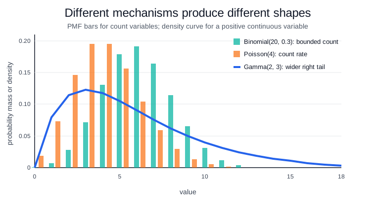
The plot instantiates the generic rows with $\mathrm{Binomial}(20,0.3)$, $\mathrm{Poisson}(4)$, and $\mathrm{Gamma}(2,3)$. The binomial and gamma examples both have mean 6, but the gamma variance is $18$ instead of $4.2$, so its right tail is much wider. The Poisson example is centered lower, near 4, and its variance equals its mean; that equality is a modeling assumption, not a universal law for count data.

Caveats

Independence, constant rate, support, and tail assumptions are part of the model. Zero inflation, truncation, seasonality, and dependence can make a convenient distribution wrong.

References

• SciPy statistics reference
• NIST Engineering Statistics Handbook: probability distributions
• OpenStax Introductory Statistics 2e, Chapter 4 introduction

Nav

Section — Probability and Statistics

← Random Variables Expectation and Variance →